13.1.9. The Channels view#

The frame buffer shows what the camera sees; the Channels view shows what the script measures and decides. A script publishes named values over the debug protocol – a temperature, a detection count, a microphone waveform, a time-of-flight depth map, or a control it wants the user to be able to change – and the IDE renders each one live as a widget, a graph, or a map in the pane below the frame buffer. Nothing has to be drawn on the image or parsed out of the terminal. On the camera side it is a few lines with protocol.CBORChannel; on the IDE side it is the Channels entry of the pane selector.

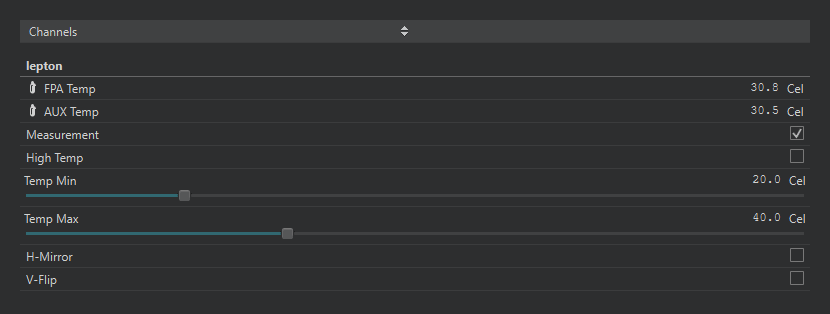
The Channels view showing a thermal camera script's controls channel: FPA and AUX temperature readouts with their unit, Measurement and High Temp toggles, Temp Min and Temp Max sliders, and H-Mirror and V-Flip toggles — A thermal camera script’s controls: two temperature readouts, toggles for the measurement modes, and sliders for the temperature range. Changing any of them sends the new value to the script.#

The view is organized by channel. Each channel the script registers becomes a section with the channel’s name as its heading, and each record in the channel becomes a row under it, in the order the script added them. When the script registers a channel or changes the shape of one, the view rebuilds itself; when the script stops, the last values stay on screen, with the controls disabled, until the next script starts.

13.1.9.1. Widgets#

Readouts and controls take the obvious forms. A label is a read-only value with its unit; a text record is a block of static rich text for headings and explanations. The writable kinds send their new value back to the script the moment you change them, where the script’s on_write callback receives the record name and value: a toggle is a switch, a slider and a spinbox set a number within the script’s range and step (the spin box for precise entry), radio buttons and a select pick one of the script’s options, a lineedit is a free-text field, and a pushbutton fires a momentary action. The view keeps your edit on screen rather than snapping it back to the camera’s last-published value while the write is in flight.

On the script side the whole set is a protocol.CBORChannel with one add per widget and a callback for the writes:

import time
import protocol
from protocol import CBORChannel

def on_write(ch, name, value):
    print(name, "=", value)      # every change lands here

ch = CBORChannel(on_write=on_write)
ch.add("Status", type="label", value="starting")
ch.add("Enable", type="toggle", value=True)
ch.add("Threshold", type="slider", min=0, max=100,
       step=1, value=50, unit="%")
ch.add("Mode", type="select",
       options=["Idle", "Track", "Record"], value="Idle")
ch.add("Calibrate", type="pushbutton")
protocol.register(name="controls", backend=ch)

while True:
    if ch["Enable"]:                   # read a control back
        ch["Status"] = "threshold %d%%" % ch["Threshold"]
    time.sleep_ms(100)

Run it and switch the pane to Channels: a section named controls appears with the five widgets, and moving the slider prints in the terminal. The other widget types – spinbox, radio, lineedit, text – are one more add each; the host protocol chapter walks through all of them.

13.1.9.2. Waveform graphs#

A waveform record is a block of interleaved samples with a sample rate – audio, accelerometer axes, an ADC trace – and the view plots it as a scrolling graph, one series per axis, named by the script. The graph controls are in its toolbar and on the plot itself:

Drag to pan and scroll to zoom; double-click to return to following the live edge. History sets how much past data is kept so you can pan back through it.
Auto Scale fits the vertical axis to the data; off, the axis is the range the script declared.
Right-click the plot to drop a marker and read the exact time and value of a sample, or to set a trigger level. With a Trigger armed the graph holds still until the signal crosses the level on a rising or falling edge – the oscilloscope way of catching a transient – and Re-arm waits for the next one.
Spectrum switches the graph to a frequency plot of the same data, with a choice of window (Hann, Hamming, Blackman, rectangular), Averaging and Peak Hold across frames, and a Log Frequency axis. The readout under the plot names the peak frequency and its level.
Pause freezes the graph without affecting a recording; Stats adds a min / max / RMS line; and the right-click menu saves the plot as an image.

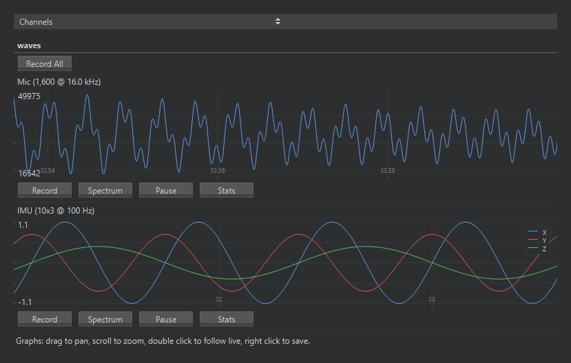
The Channels view with two waveform records scrolling live: a 16 kHz microphone trace and a three-series accelerometer trace with its X, Y, and Z legend, each with its Record, Spectrum, Pause, and Stats buttons — Two waveform records scrolling live: a microphone trace and a three-series IMU trace.#

A waveform field takes the sample rate and, for several signals at once, the number of interleaved series and their names; each update is the raw bytes of an array of samples in the field’s typecode:

import math
import time
import protocol
from array import array
from protocol import CBORChannel

RATE, CHUNK = 1000, 100            # 1 kHz, 100 ms per update

ch = CBORChannel()
ch.add("IMU", type="waveform", sample_rate=RATE, series=3,
       typecode="f", min=-2.0, max=2.0,
       options=["X", "Y", "Z"], unit="g")
protocol.register(name="signals", backend=ch)

t = 0
while True:
    block = array("f")
    for i in range(CHUNK):
        phase = 2 * math.pi * 2 * (t + i) / RATE
        block.extend((math.sin(phase), math.cos(phase), 1.0))
    ch["IMU"] = bytes(block)        # interleaved X, Y, Z
    t += CHUNK
    time.sleep_ms(100)

13.1.9.3. Depth maps#

A depth record is a grid of distances – the frames a time-of-flight sensor produces – and the view draws it as a false-colour map scaled up to the graph height. The toolbar chooses the rendering: the palette (the camera’s own Depth, Rainbow, and Ironbow palettes, plus light and dark palettes for event cameras), the scaling filter that enlarges the small sensor grid (bicubic for a smooth surface, bilinear, or nearest for one block per sensor pixel), and the tone mapping that turns distance into colour: Script Range uses the range the script declared, Auto Range stretches the colours over the distances actually present in each frame (ignoring the outlying few percent), and Equalize spreads them over the frame’s distribution so a flat scene still shows its detail. The header reports the map’s size, the declared range, and the frame’s minimum, maximum, and mean; hovering over the map reads out the distance under the cursor, and Save Image writes the rendered map to a PNG.

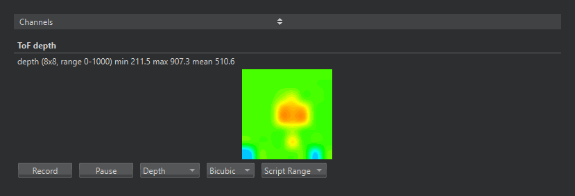
The Channels view showing an 8 x 8 time-of-flight depth map scaled up smoothly with the Depth palette, the palette, scaling, and tone-mapping selectors in its toolbar, and the header reporting the size, declared range, and the frame's minimum, maximum, and mean — A time-of-flight depth map of a hand in front of the sensor, with the palette, scaling, and tone-mapping selectors in the toolbar.#

A depth field declares its grid size and range; each update is the grid as packed 32-bit floats, which is what the tof module’s reader produces:

import struct
import time
import tof
import protocol
from protocol import CBORChannel

tof.init()
ch = CBORChannel()
ch.add("depth", type="depth", width=tof.width(),
       height=tof.height(), min=0, max=1000)
protocol.register(name="ToF", backend=ch)

while True:
    try:
        d, dmin, dmax = tof.read_depth(vflip=True, hmirror=True)
    except RuntimeError:
        continue
    ch["depth"] = struct.pack("<%df" % len(d), *d)
    time.sleep_ms(50)

13.1.9.4. Recording#

Every graph and map has a Record button, and a channel with more than one of them has a Record All bar that starts them together. Recording writes the data as it arrives – not the rendering – to a file whose format follows the extension you pick in the save dialog: CSV for spreadsheets and plotting tools, WAV for single-channel audio waveforms, NumPy .npy arrays for Python, and Edge Impulse JSON or CBOR for uploading straight into an Edge Impulse project as training data, with an optional label that names the files. Only the formats that can hold a record’s data are offered; a depth map, for example, cannot be a WAV file. A long capture is split into numbered parts so no single file grows unwieldy, and a recording survives the script re-registering its channels. The readout beside the button tracks how many samples have been written and the file size.

The pane’s Channel Polling interval, in the protocol section of the preferences, sets how often the IDE asks the camera for new channel data; the default suits scripts that publish a few times a second, and a script streaming audio benefits from a shorter interval.